Semester Project by Loïs Bilat at VITA Lab – EPFL – Fall 2019
Supervised by Alexandre Alahi and Brian Sifringer.
GitHub · Intro slides · Midterm slides · Final slides
---/
Introduction
Description of the problem
The quality of audio recordings from a mobile device has gotten better over the years, but there are still a lot of factors that can decrease the quality. Among others, the size and the quality of the microphone sensor, as well as its location relative to the audio source can have a non negligable impact. We also cannot forget potential ambient noise (e.g. voices, rain, traffic) and reverberation that can be caused by the size and shape of the room.
It would be useful if we could somehow correct all those issues by using software tools that could take a low quality audio file, and improve it as if the audio was recorded using high quality equipment in a perfectly silent environment. More precisely, given a music sample of any length and recorded using low quality equipment in a noisy environment (therefore it might have a low resolution, some noise and some reverberation), we want to output a higher resolution version of the same audio sample, with some of the noise and reverberation removed. If the resulting music file sounds better to the human ear than the original, the transformation is considered successful.
Why is it important?
If we want high-quality recording on our mobile devices, we need some software solutions, as we might not be able to improve the hardware quality of the microphone due to physical limitations. It is also hard to control the environment where we want to do our recording. This type of technology could then be used by smartphone manufacturers to let the users create studio-grade quality recordings.
Moreover, if we are able to improve the quality of an audio signal, we might also be able to improve the quality of other types of signal (e.g. an electromagnetic signal). For instance, it could be used to improve the precision of the LIDAR technology that can be very useful for autonomous cars.
Goal of the project
Most of the research on audio denoising is done on speech, as it is probably the domain where such techniques might be the most useful (intelligent assistants, speech-to-text, etc). Therefore, there are very few papers that tried these techniques on music, and when they did it was often as an afterthought, and not the primary goal of their project.
The goal of this project was to study the state-of-the-art in audio denoising and super-resolution, and then improve it by adding some other ideas coming from image processing research. At the time of the start of the project, the state of the art in speech super-resolution seemed to be Speech Denoising with Deep Feature Losses (complete reference at the end), and the state of the art for speech denoising seemed to be Adversarial Audio Super-Resolution with Unsupervised Feature Losses. The plan was to first implement this second paper as a baseline, and then try to improve it. Unfortunately, it proved more challenging than expected to implement this model, as some details were not clear enough to implement it correctly.
Therefore, the paper Audio Super-Resolution using Neural Nets was chosen as a baseline for this project, as the paper was very clear and a github repository was also available for more details.
Model
The model proposed here is a convolutional autoencoder with skip connections, also known as U-net. Starting from this base model, a few improvements were then added, such as a discriminator network to transform the model into a GAN and another autoencoder to further improve the learning process.
After this, techniques like Collaborative GAN, Conditional GAN and Patch GAN were also implemented.
Original model
Architecture
The original architecture is, as mentioned before, a convolutional autoencoder with skip connections. It consists of $B$ downsampling blocks, one bottleneck block, $B$ upsampling blocks and a final convolutional layer. There are stacking residual connections between a downsampling and an upsampling block at the same level, and an additive residual connection between the input and the final block.
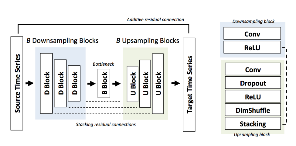
Each downsampling block consists of a convolutional block, and a ReLU block. These have a stride of 2, the number of channels outputed by each convolutional block is given by the array [126, 256, 512, 512, 512, ...], and the size of filters is given by the array [63, 33, 17, 9, 9, 9, ...]. The ReLU block is more precisely a Leaky rectified linear block with a slope of 0.2 on the negative side.
The bottleneck block is the same as a downsampling block, but with a dropout with probability 0.5 after the convolutional layer.
In the upsampling blocks, the convolutional layer uses the same filter sizes as the downsampling blocks, but in reversed order. The number of channels outputed by the convolution is double the one in the corresponding downsampling block, and we have a stride of 1. We then have a dropout of 0.5 and a LeakyReLU with a slope of 0.2. Following this, we have the DimShuffle operation, more precisely the Sub-pixel operation, that takes some data of shape $N\times C \times W$ and transform it into data of shape $N\times C/2 \times 2W$ by interleaving elements from two channels together.

Finally, we have the stacking block that takes the output of the corresponding downsampling block and concatenates it on the channel dimension with the output of the sub-pixel block.
After all the upsampling blocks, we finish with a final block that makes of convolution with 2 outputs channels, a filter size of 9 and a stride of 1, then the subpixel operation (this will reshape our data so that we are left with only one channel), and then we add the output of this to our input data to get the output of the network (this is the additive skip connection). What this connection implies is that the network doesn’t learn how to create denoised sound directly, but rather it learns how to create “denoising data” that when added to the audio itself improves it.
To better understand this architecture, you can see here a schema of the network:
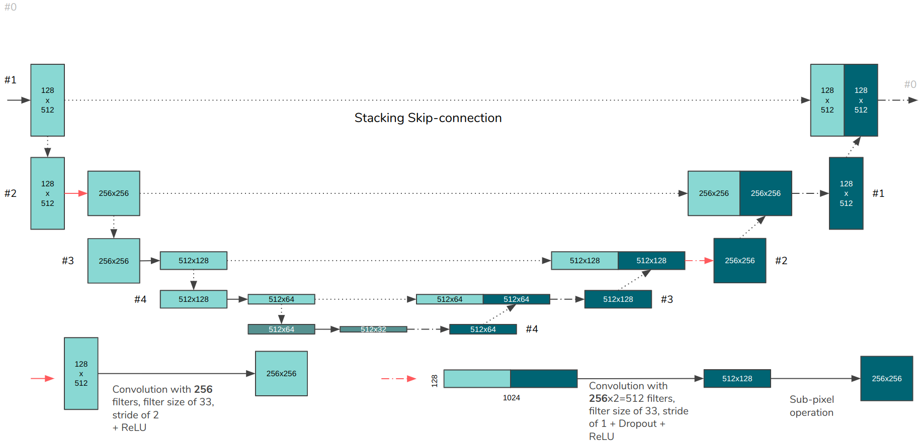
Moreover, you can see here for a toy example with depth 4 and where inputs have shape (1, 1024), what are the sizes of each layer and the parameters of the convolution.
           input : (1, 1024) -----------------------------------------
                                                                     |
        (1, 1024)->conv(128,63,2)->(128, 512)-------------------     |
                                                               |     |
      (128,512)->conv(256,33,2)->(256, 256)---------------     |     |
                                                         |     |     |
    (256,256)->conv(512,17,2)->(512, 128)----------      |     |     |
                                                   |     |     |     |
  (512,128)->conv(512,9,2)->(512, 64)---------     |     |     |     |
                                             |     |     |     |     |
(512,64)->conv(512,9,2)->(512,32)            |     |     |     |     |
                                             |     |     |     |     |
  (512,32)->(512x2,9)->(1024,32)-sp->(512,64):     |     |     |     |
                                             =     |     |     |     |
                                         (1024,64) |     |     |     |
                                                   |     |     |     |
    (1024,64)->(512x2,9)->(1024,32)-sp->(512,128)--:     |     |     |
                                                   =     |     |     |
                                               (1024,128)|     |     |
                                                         |     |     |
      (1024,128)->conv(256x2,33)->(512,128)-sp->(256,256):     |     |
                                                         =     |     |
                                                     (512,256) |     |
                                                               |     |
        (512,256)->conv(128x2,63)->(256,256)-sp->(128,512)-----:     |
                                                               =     |
                                                           (256,512) |
                                                                     |
           (256,512)->conv(2,9)->(2,512)-sp->(1, 1024)---------------+
                                                                     =
                                                                 (1, 1024)
Training
We train this network using the $L2$ loss
$$\mathcal{L}G = \mathcal{L}{L2} = \frac{1}{W}\sum_{i=1}^W \left|x_{h,i} - G(x_l)_i\right|$$
where $x_h$ is the high quality audio signal, and $x_l$ the low quality signal.
It is also possible to use the $L1$ loss
$$\mathcal{L}G = \mathcal{L}{L1} = \frac{1}{W}\sum_{i=1}^W |x_{h,i} - G(x_l)_i |$$
by simply changing a parameter in the command.
GAN
To transform our system into a Generative Adversarial Network (GAN), we need to add a discriminator network, whose goal is to classify given samples as real or fake. In our case, we want that the original high quality audio should be classified as real, and the generated improved audio should be classified as fake. The goal of our first network, called generator here, is to create improved samples that will be classified as real by the discriminator.
The architecture of the discriminator is basically the first half of the generator network, with a Batch normalization layer added between the convolutional and ReLU layers. At the end, everything is sent into a linear layer and a sigmoid activation function that will output one value between 0 and 1, the probability that a given sample is real. This Discriminator is trained with the following loss function
$$\mathcal{L}_D = - [\log D(x_h) + \log(1-D(G(x_l)))]$$
When training the model, we first train the generator by itself for a while, and then we start training the discriminator and we change the generator loss $\mathcal{L}_G$ to
$$\mathcal{L}G = \mathcal{L}{L2} + \lambda_{adv}\mathcal{L}_{adv}$$
with
$$\mathcal{L}_{adv} = - \log D(G(x_l))$$
meaning that the generator will not only look at its own loss (i.e. how far are we from the target sample), but it will also try to generate more realistic samples to fool the discriminator.
Autoencoder
To improve the model further, we added another network, with an autoencoder architecture, that will also contribute to the loss function of our generator by computing the distance between our generated and target data, but in the latent space created at the bottleneck of this autoencoder. The architecture is the same as the generator, but the residual connections are removed (and therefore some parameters for the number of channels and filters are adapted consequently). Moreover, batchnorm layers are added in the downsampling block as initial testing showed that otherwise values were getting extremely small in the bottleneck, and this was causing some issues.
This autoencoder is trained using the $\mathcal{L}_{L2}$ loss, on the identity task (meaning that the target is the same as the input). The goal of this is to find a lower dimension representation of our data (at the bottleneck), that can give some useful information to our optimization problem.
The loss for the generator is now
$$\mathcal{L}G = \mathcal{L}{L2} + \lambda_{adv}\mathcal{L}_{adv} + \lambda_f \mathcal{L}_f$$
with
$$\mathcal{L}f = \frac{1}{C_f W_f} \sum{c=1}^{C_f} \sum_{i=1}^{W_f} \left| \psi (x_h){i,c} - \psi(G(x_l)){i,c}\right|$$
where $\psi(x)$ is the output of the network at the bottleneck layer, and $C_f$ and $W_f$ are the number of channels and the width of the data at the bottleneck.
Collaborative GAN
In a normal GAN architecture, once the model is trained, we only use the generator to create our final samples. Collaborative GAN is a technique where the discriminator is also used during the sampling phase, to hopefully get better results. Collaborative GAN is used only once the original training of the model is completely done. I will present here the modified version of this method, adapted from the original paper.
There are two main parts to this method:
Collaborative sampling
This step happens when you want to generate a sample, but also want to improve it using information provided by the discriminator. Since this happens after the training, we want to freeze the parameters of both the generator and the discriminator.
Suppose we have an input sample, i.e. a low quality audio sample. We send it as an input to the generator, to generate an improved version. We then take the output, and give it to the discriminator. If the discriminator classifies it as “real” with a high enough confidence (in the code 0.5 is used, but higher values may be required for better results), we stop, as we consider our sample is good enough. However, if our sample is classified as “fake”, we will try to improve it. This is illustrated here:
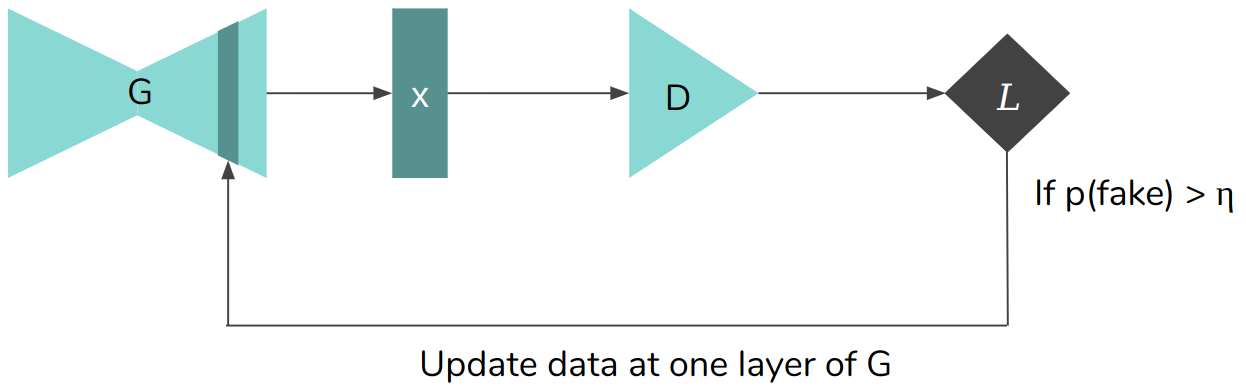
For this, we will look at the internal activations of the generator network, in particular the activations at one layer (we call it $x_l$). $x_l$ corresponds to the activation at the output of the $l$th upsampling block of our generator. We then compute the gradient of this tensor of activations relative to the loss of the discriminator, and then update the value of $x_l$ by gradient descent. The values of $x_l$ are then once again propagated to the end of the network, which will give us a new sample. (Note that during this second pass with the modified $x_l$, the values provided by the skip connections come from the original propagation of x.)
Finally, we repeat this while our sample is not classified as “real” by the discriminator. We still stop after a maximum number of iterations to not spend too much time with problematic samples.
To sum up:
- Compute $y = G(x)$, a generated sample
- Compute $p = D(y)$, the confidence of the sample being “real”
- If $p < \eta$:
- Compute the gradient $\frac{d \mathcal{L}_D}{d x_l}$, where $x_l$ is the internal activation at layer $l$ of the upsampling blocks.
- Update $x_l$ by gradient descent, i.e. $x_l = x_l - \lambda \frac{d \mathcal{L}_D}{d x_l}$
- Do another forward pass $G(x)$, but when reaching layer $l$, replace the values by the new value of $x_l$.
- Continue the forward pass until we have a new generated sample.
- If it is still classified as “fake”, and we have not reached the maximum number of iterations, repeat.
- If $p > \eta$: we have our sample, nothing else to do.
This whole algorithm is done at the complete end of our pipeline, when we generate samples for our output audio file.
However, our discriminator, despite being able to classify samples as real and fake, is not really capable of helping the refining process. For this reason, we have to train it beforehand. This step is called discriminator shaping.
Discriminator shaping
Discriminator shaping happens after the normal training, but before the generation of the final audio file using collaborative sampling. It works as follows:
For a given number of iterations, and given a pair $(x_l, x_h)$ of low quality and high quality audio, we train the discriminator with $x_h$ given as “real” data, and the collaboratively sampled data generated from $x_l$ as “fake” data.
Conditional GAN
Another technique that can be used to improve the results of our model is conditional generative adversarial network (also known as CGAN). This technique is for instance used by pix2pix, where the goal is to transform an image into another (often starting from a schematic image, i.e. only the borders, or maybe a segmentation map, and trying to create a realistic image corresponding to this input).
This was implemented in this project since this idea (image to image instead of random latent data to image) is actually quite similar to what we are trying to do here. Indeed, we already start from an image, and therefore this model might be more appropriated than the usual generator model.
The basic idea of CGAN is this: You take the same model as for our previous GAN (a generator, and a discriminator that takes improved samples and classifies them as real or fake), but you edit the discriminator so that it takes both the improved data, but also the original data as an input (we simply concatenate them on the channel dimension).
This change means that now the goal of the discriminator is to ask “Is this a real-sounding improved sample, given what the original data is?”, instead of only “Is this a real-sounding improved sample?” (therefore the name conditional GAN).
You can see here an illustration of this change, taken from the original pix2pix paper.
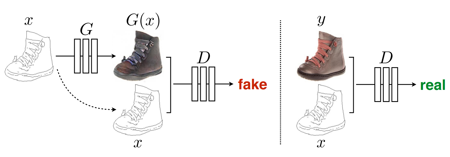
Here they use images, but the idea is the same. Your input x (the drawn shoe, respectively the low quality audio file) is given to the generator to create an improved version (the gray shoe / improved audio). Then, you give both the generated sample (gray shoe / improved audio) and the original data (drawn shoe / low quality audio) to the discriminator. Moreover, when training the discriminator, you will also give two samples as the input, namely the original image (drawn shoe / low quality audio) and the target image (brown shoe / high quality audio).
The architecture for this conditional discriminator is exactly the same as the original discriminator, with simply a different input shape. The rest of the network doesn’t change.
Preprocessing
Since this model should work with any audio file provided, we need to do some preprocessing beforehand. There are two parts for this.
Audio degradation
Since the goal of this project is to improve audio quality, we need to create our dataset. We use the MAESTRO Dataset (as described later), which consists of only high quality audio files. We therefore need to degrade those files to have our training data pairs. Three types of preprocessing are supported: Noise, Downsampling and reverberation. All of those are done using the sox library, and can be chained together.
For the downsampling, we have two arguments, target_res and input_res. If we name our pair of input/output data samples (x, y), we can create y by simply downsampling our audio to target_rate. To create x, we first downsample our data to input_res, and then upsample it to target_rate using simple linear interpolation. We do it this way so we can have a symmetrical network, which is necessary for our skip connections to work properly.
Audio split
Since our network takes as input some data with a given size, we need to split our original audio file into multiple small segments. We do this using a sliding window with a stride (usually a window of 2048 and a stride of 1024). This gives us some redundancy in the data, and this way any part of the music is seen twice, at a different position in the input.
During the evaluation phase, when we want to reconstruct an audio file, we need to put samples of the music back together. The naive way would be to split the audio file using a stride of the same value as the window size (i.e. no overlap), improve each sample individually, and then concatenate all the blocks together. This, however, doesn’t give us good results, and we can hear a distinctive noise at the junction between two samples. This happens because our network handles the border of a sample differently than data in the middle of the sample (we have to use some padding on the border, so the sound is distorted).
Therefore, for the evaluation phase, we still split the data using a sliding window with some overlap. When putting the blocks together, we will only keep a part of each sample, and the borders will be cropped. This can be seen in the following illustration.
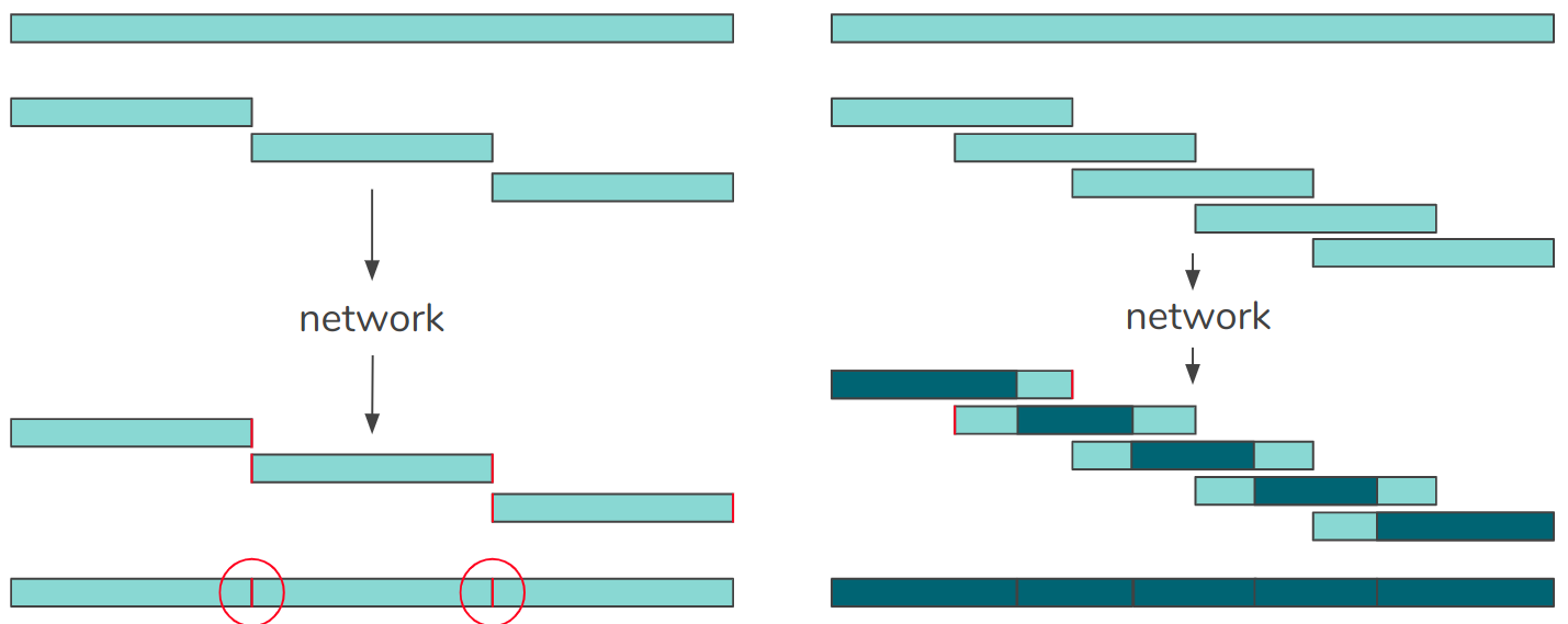
With this technique, we don’t have any audio artifact at the junction between two samples.
Code
You can find on this GitHub page all the code used for this project. Required libraries:
matplotlib
torch
torchaudio
numpy
pandas
graphviz
How to run
usage: main.py [-h] [-c COUNT] [-o OUT] [-e EPOCHS] [-b BATCH] [-w WINDOW] [-s STRIDE] [-d DEPTH] -n NAME
               [--dropout DROPOUT] [--train_n TRAIN_N] [--load LOAD] [--continue CONTINUE]
               [--dataset DATASET] [--dataset_args DATASET_ARGS] [--data_root DATA_ROOT]
               --rate RATE --preprocessing PREPROCESSING [--loss LOSS] [--gan GAN] [--ae AE]
               [--ae_path AE_PATH] [--collab COLLAB] [--cgan CGAN] [--lr_g LR_G] [--lr_d LR_D]
               [--scheduler SCHEDULER]

optional arguments:
  -c COUNT         number of mini-batches per epoch [int], default=-1 (use all data)
  -o OUT           number of samples for the output file [int], default=500
  -e EPOCHS        number of epochs [int], default=10
  -b BATCH         size of a minibatch [int], default=32
  -w WINDOW        size of the sliding window [int], default=2048
  -s STRIDE        stride of the sliding window [int], default=1024
  -d DEPTH         number of layers of the network [int], default=4, maximum allowed is log2(window)-1
  -n NAME          name of the folder in which we want to save data for this model [string], mandatory
  --dropout        value for the dropout [float], default=0.5
  --train_n        number of songs used to train [int], default=-1 (use all songs)
  --load           load already trained model to evaluate [string], default=''
  --dataset        type of the dataset [simple|type], default=simple
  --dataset_args   optional arguments for specific datasets, strings separated by commas
  --data_root      root of the dataset [path], default=/data/lois-data/models/maestro
  --rate           sample rate of the output file [int], mandatory
  --preprocessing  preprocessing pipeline string with each step separated by a comma
  --loss           loss for the generator [L1, L2], default='L2'
  --gan            lambda for the gan loss [float], default=0 (disabled)
  --ae             lambda for the autoencoder loss [float], default=0 (disabled)
  --ae_path        path to the trained autoencoder model
  --collab         enable the collaborative GAN [bool], default=False
  --cgan           enable Conditional GAN [bool], default=False
  --lr_g           learning rate for the generator [float], default=0.0001
  --lr_d           learning rate for the discriminator [float], default=0.0001
  --scheduler      enable the scheduler [bool], default=False
For instance, the following command:
main.py --count -1 --out 1000 -e 10 --batch 32 --window 2048 --stride 1024 \
        --depth 8 --train_n -1 --name gan_10 --data_root /data/lois-data/models/maestro \
        --rate 10000 --lr_g 0.0001 --lr_d 0.0001 --gan 0.0001 \
        --preprocessing "sample 5000 10000"
will run the model for 10 epochs, using minibatches of 32 samples. The network will have a depth of 8, and we split the data into sub-samples of 2048 of width, with some overlap (stride of 1024). We train on all available training data, but create an improved version for only one output file. Our data is stored in the /data/lois-data/maestro folder. Our target rate is 10kHz, the learning rate for both the generator and the discriminator is 0.0001, the lambda for the discriminator part of the composite loss is 0.0001. Finally, we want to do some upsampling from 5kHz to 10kHz.
Note that you need to create an out folder inside the src directory. All the results will be saved inside.
If you want to use the autoencoder, you first have to train it separately using the ae.py file:
usage: ae.py [-h] [-c COUNT] [-o OUT] [-e EPOCHS] [-b BATCH] [-w WINDOW] [-s STRIDE] [-d DEPTH]
             -n NAME [--dropout DROPOUT] [--train_n TRAIN_N] [--dataset DATASET]
             [--data_root DATA_ROOT] --rate RATE [--loss LOSS] [--lr_ae LR_AE] [--scheduler SCHEDULER]
The resulting model archive can then be used in the main program by giving its path to the --ae_path argument.
Preprocessing options
- Downsample:
"sample low_res high_res"— creates input atlow_resHz and target athigh_resHz. Set--ratetohigh_res. - Noise:
"noisetype variance volume"—noisetypecan bewhitenoise,pinknoise,brownnoise, ortpdfnoise. Good volume values are around 0.001. - Reverberation:
"reverb variance reverberance hf_damping room_scale stereo_depth pre_delay wet_gain=0"
Chain multiple steps with commas: --preprocessing "sample 5000 10000,whitenoise 0 0.002"
Evaluation
By default, once the model has finished training, it will take a file and try to improve it. This file will be out.wav. If you want to evaluate other files, run the original command with --load filename added, where filename is relative to --data_root. This will look for a model save at out/name/models/model.tar.
Code structure
main.py—init(): argument parsing ·init_net(): initialize networks ·load_data(): preprocess files, load to memory, return dataloaders ·pipeline(): train/evaluate model, create output filetrain.py—train(): training loop with plots ·make_train_step(): one training steptest.py—test(): test loop ·make_test_step(): one test stepnetwork.py—Generator,Discriminator,AutoEncoder,ConditionalDiscriminatorclassesfiles.py—SimpleFiles,MAESTROFilesdataset representationsdatasets.py—AudioDataset: PyTorch dataset returning (input, target) pairspreprocessing.py—preprocess(): given filename and chain, returns output filenames ·sample,noise,reverbimplementationsutils.py— shared utility functionsmetrics.py— metric implementations called after trainingae.py— autoencoder training code
Experiments
MAESTRO Dataset
This dataset consists of more than 200 hours of recorded piano, in high quality (44.1kHz), and in the wav format. Each file is also available in MIDI format, but those were not used as we wanted to use some more realistic data. Due to the huge amount of data, not all of it was used.
It was the highest quality data that we found, but it had the problem of having a little bit of background noise (since it was recorded in a concert hall, you can hear people moving chairs and so on).
Metrics
To measure the performance of the model, the log-spectral distance (LSD) is used:
$$LSD(x,y) = \frac{1}{L} \sum_{l=1}^L \sqrt{\frac{1}{K} \sum_{k=1}^K (X(l,k) - \hat{X}(l,k))^2}$$
where $X$ and $\hat{X}$ are the log-spectral power magnitudes of $y$ and $x$, respectively, defined as $X=\log{\left| S\right|^2}$ where $S$ is the short-time Fourier transform (STFT) of the signal. $l$ and $k$ index frames and frequencies. Frames of length 1024 were used.
We compute the baseline LSD between the low quality and high quality signal:
$$LSD_{baseline} = LSD(x_{low}, x_{high})$$
Then for each model version:
$$LSD_{version_x} = LSD(x_{improved_by_version_x}, x_{high})$$
The version with the smallest distance is better.
We also use the Signal-to-Noise ratio (SNR):
$$SNR(x,y)=10\times\log_{10}\left(\frac{| y |_2^2}{| x-y |_2^2}\right)$$
This is the difference between $x$ and $y$, normalized and converted to decibels. Higher is better.
Results
For all experiments: super-resolution from 5kHz to 10kHz, no noise added. Approximately 1.4 GB of raw data (~2 hours of music). Data split into samples of length 2048 with overlap 1024. Network depth 8. Each experiment runs for 5 epochs, minibatch size 32, L2 generator loss.
Original data
Low quality audio (input to improve):
High quality audio (target):
As you can hear, the degradation in the first file is clear. It sounds like it was recorded in a box, and it is due to the loss of high frequencies following the down-sampling of the file.
Scheduler
Before we take a look at the results, it is important to talk about something that was implemented but ultimately not used: a scheduler.
The idea behind the scheduler is the following; we start with given learning rates and train our model, and regularly reduce the learning rate to avoid leaving good minima by “moving too much”. The ReduceLROnPlateau scheduler was chosen here. We can see a comparison in the loss curves:
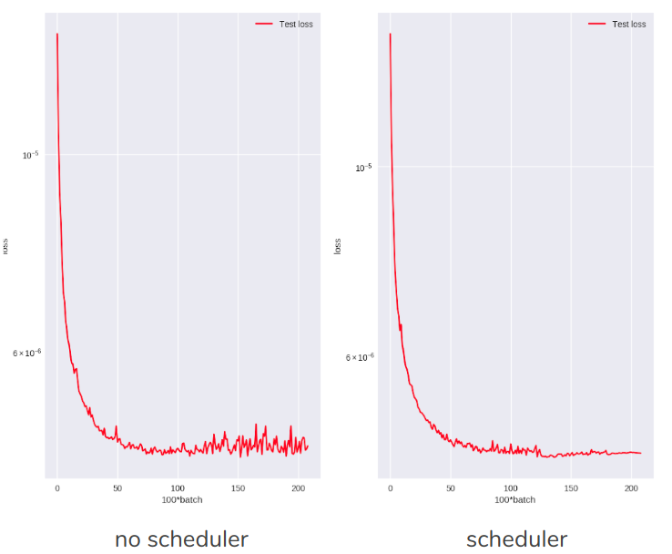
The version with the scheduler seems better, or at least it is more stable and less noisy after a while. However, if we look at the LSD and SNR metrics, we can see that the version without the scheduler gives better results.
| $LSD_{baseline}$ | $LSD_{no\ scheduler}$ | $LSD_{scheduler}$ |
|---|---|---|
| 2.2235 | 1.6079 | 1.6777 |
| $SNR_{baseline}$ | $SNR_{no\ scheduler}$ | $SNR_{scheduler}$ |
| 28.8033 | 1.70355 | 1.70319 |
A notable problem: $SNR(low\ res, high\ res)$ will always be better than $SNR(improved, high\ res)$. This means the metric will not be useful to tell us if we beat the baseline, though it can still compare two models against each other.
The scheduler is disabled for the remaining experiments.
Baseline model
Low quality audio (input):
Audio generated by the base network:
High quality audio (target):
It is unfortunately hard to hear an improvement. It is very subtle, but we could say that the notes are “sharper” than in the low quality file. If we compare the low quality with the high quality, we can hear that the higher notes get quieter in the low resolution. This is partially fixed in the improved version, where the higher notes get louder again.
| $LSD_{baseline}$ | $LSD_{base\ network}$ |
|---|---|
| 2.2662 | 1.5919 |
| $SNR_{baseline}$ | $SNR_{base\ network}$ |
| 28.8033 | 1.7032 |
If we take a look at the training loss, we can see that it is useless to have a high number of epochs, as we are already in a plateau after 4 epochs.
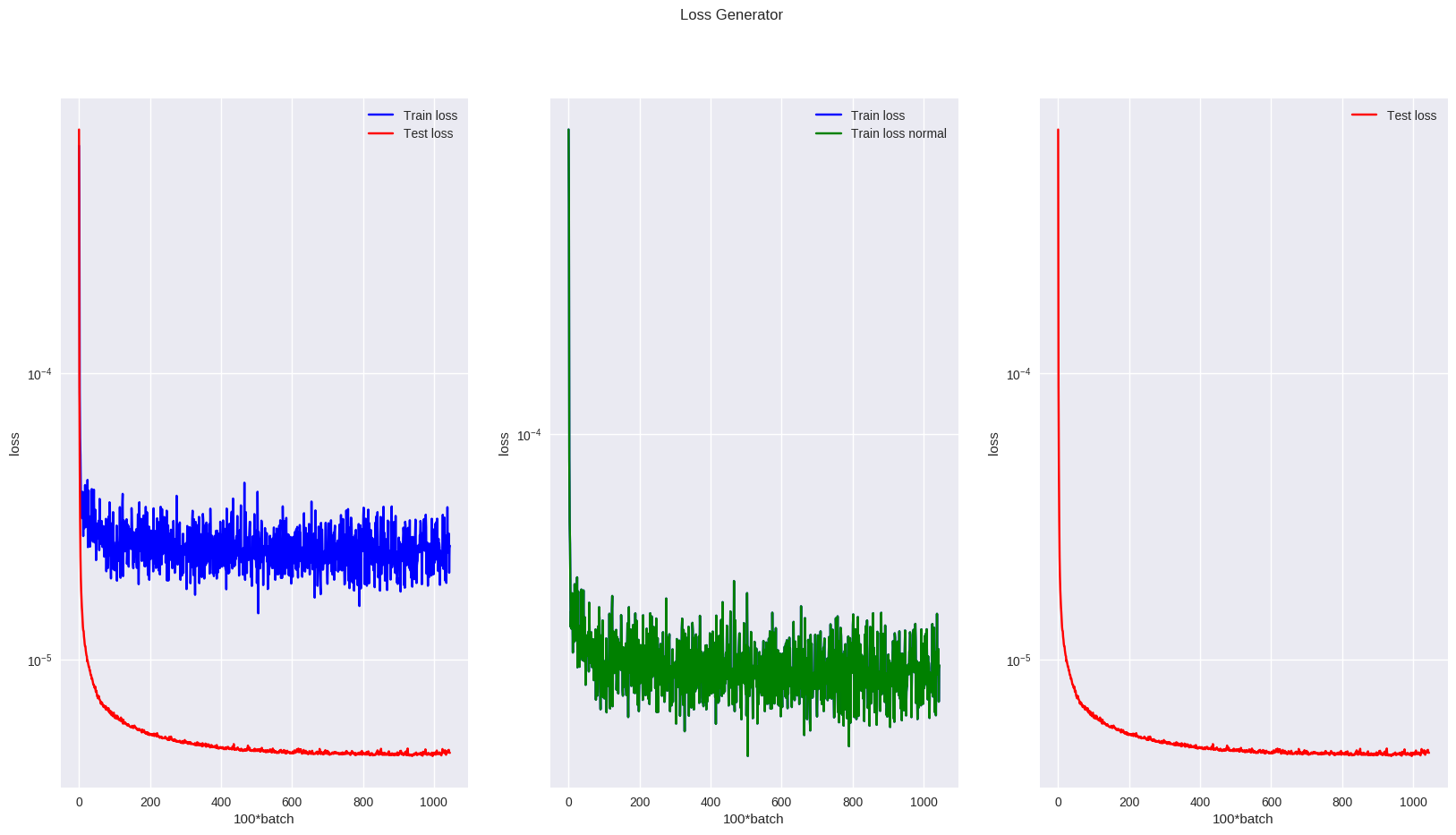
The middle graph corresponds to the training loss averaged over the last 10 mini-batches. On the right is the test loss, evaluated every 10 mini-batches on 4 minibatches from the test file. The reason why the test loss is lower than the train loss is because the dropout layers are disabled when evaluating the network, therefore giving a better result.
A second experiment was done by increasing the size of the sliding window to 4096 (stride 2048):
Base with samples of 2048:
Base with samples of 4096:
We can hear that the version with samples of 2048 sounds better, as the other one has some saturation in the high notes.
However a problem appears if we look at the metrics:
| $LSD_{baseline}$ | $LSD_{2048}$ | $LSD_{4096}$ |
|---|---|---|
| (2.2662) | 1.5919 | 1.3184 |
| $SNR_{baseline}$ | $SNR_{2048}$ | $SNR_{4096}$ |
| (28.8033) | 1.7032 | 1.7024 |
The better-sounding audio has a higher LSD, which shouldn’t be the case if our metric accurately represented hearing quality. This probably happens because the saturation is considered “high frequency data” and is taken into account by the LSD. This is problematic, since it means we cannot completely rely on the LSD to compare samples, and human opinion is clearly necessary.
We can see an illustration of this here, where the spectrogram of each file is shown. First, the difference between the input (left) and target file (right):
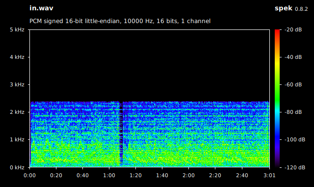
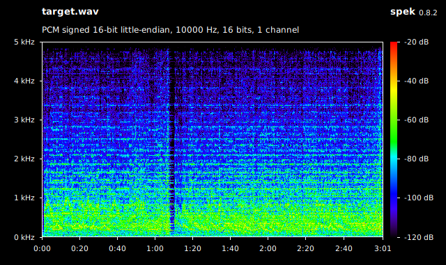
We can see the high frequency cutoff at 5kHz. Now, comparing the two generated files — 2048 (left) vs 4096 (right):
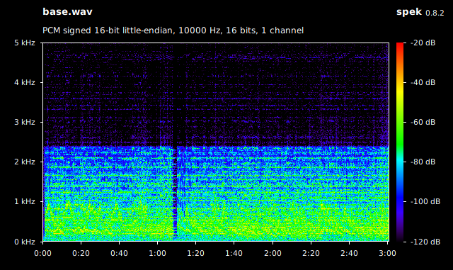
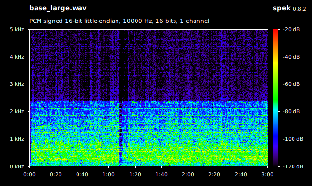
With 2048 (left), higher frequencies are added but with very low intensity. With 4096 (right), more frequencies reach up to 5kHz — the symptom of the saturation we hear.
From now on, we will use a sample width of 2048.
Autoencoder
Here, the additional autoencoder network was added with a lambda of 0.0001.
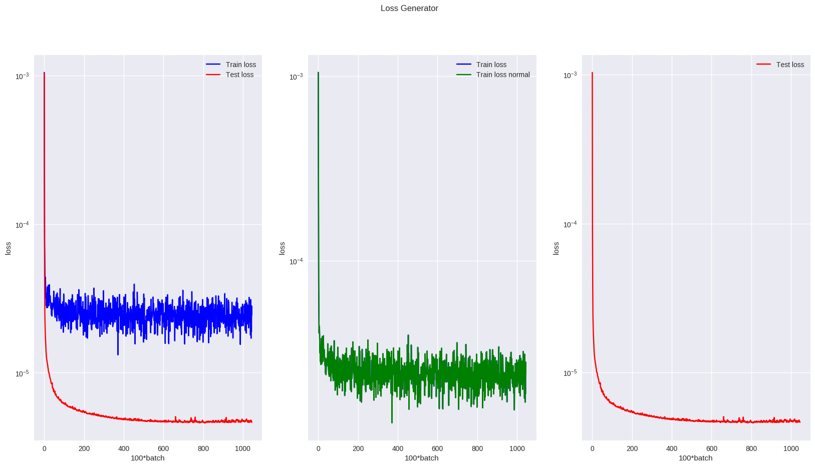
This represents the loss for the generator. Both the composite loss (blue) and the generator-only loss (green) are drawn. The lambda for the autoencoder is small, so they look nearly identical.
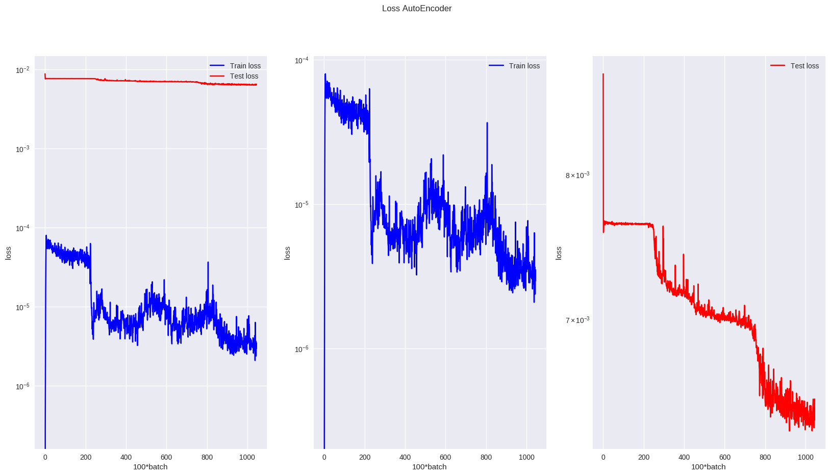
This represents the loss of the autoencoder. The training loss corresponds to the loss at the bottleneck during training, whereas the test loss corresponds to the MSE on the identity task output. (The large jump at the beginning should be ignored — it only happens because in the first iterations the autoencoder is not yet used.)
We can clearly see that the autoencoder is doing something. Its loss on the identity task is decreasing, and the loss at the bottleneck is also decreasing, which seems to indicate that the generator is integrating information from the autoencoder.
| $LSD_{base\ network}$ | $LSD_{ae}$ |
|---|---|
| 1.5919 | 1.5706 |
| $SNR_{base\ network}$ | $SNR_{ae}$ |
| 1.7032 | 1.70292 |
Base model:
Autoencoder model:
Here you can hear/see the main problem that will occur in all the following tests: the metrics are very close, sometimes contradictory, and not exactly reliable as seen before, and a hearing test doesn’t give us any information as the results are extremely close.
Something that can be tried to improve the results with the autoencoder:
- Train longer — we see in the autoencoder loss that we clearly aren’t in a plateau, so there is still room for improvement.
- Increase the lambda — in the generator graph, we see that the composite loss is basically the same as the generator-only loss. This implies that the autoencoder information is almost not present in the final gradient, and increasing it might be better.
GAN
Unfortunately, the GAN wasn’t working. The discriminator’s loss always stayed very high, and no combination of parameters were found to make it work.
Therefore, there are no results to show for the GAN, and neither for the collaborative and conditional GANs.
Discussion
When creating a neural network, one important aspect is to choose the appropriate loss. There are a few types of losses that can be considered.
Reconstruction loss — This one is the simple loss that we usually think of at first. It looks at how far away we are from the target data, in a “mathematical” way. We often use the mean squared error, but other types of distance exist.
Perceptual loss — This one looks at the distance between two signals, but at a higher level. For instance, we can look at the difference in frequencies between the two signals. We still compute the loss between two accurate representations of the data, but we look at it from a different angle. We could have for instance used the Log-spectral distance (LSD) used in the metrics, and it might have been helpful, especially for super-resolution where it is important to recreate high frequencies.
Adversarial loss — This is the one implemented by the discriminator. The adversarial network tries to learn that the generator creates fake samples, and meanwhile the generator tries to create samples that are classified as real by the discriminator. This is a kind of minimax game.
Style loss — Often used in image processing to create images “in the style of” another image. It looks at very high-level features of the data. In the context of this project, style loss doesn’t seem very useful — the style of a music file would be something like the pace, the tonalities, the rhythm, the instruments, or the composer. However here this is basically the same for all the data, as all of it is classical music. On the other hand, if we were to expand this project to different types of music, it could be useful to prevent the generated audio from sounding too different (e.g. if the input is a guitar melody, you don’t want it to sound like a violin after removing the noise).
The idea behind the additional autoencoder is actually to try to automatically find those specific losses. It tries to find a low dimension representation of the data, which could be anything from just a low resolution version of the audio, or features about “sadness”, “color”, or “speed” of the music. Since the architecture of this autoencoder is still quite simple, it is probable that it is not able to learn such complicated features.
There is also the problem of hyperparameter tuning. For the base model, there are already a lot of parameters to choose: the window size, architecture details (dropout rate, LeakyReLU slope), the number of layers, the learning rate. As soon as we add the discriminator, we double the number of parameters, plus what weight to give the discriminator in the composite loss.
If we want to find the best parameters, we would have to add additional code and use a validation dataset. The problem is not the code or the dataset, but finding which metric to use to decide what parameters are best. Ideally we would need to use human opinion, as it is the most important metric for this task, but it would be impossible to integrate this into an automatic process. We are left with mean square error or log-spectral distance, but it’s hard to know which one is the closest to what a person would perceive.
Conclusion
Audio denoising is a very complicated task, and as we have seen with the results, it is really hard to get an output that really sounds better. Unlike with images and videos, where a little artifact or defect will maybe go unseen by the untrained eye, something similar in an audio file is immediately noticeable, especially with music with little variation (everybody knows what a piano is supposed to sound like, so any variation will be noticeable). With more general sound, like speech mixed with background music, it can maybe be less problematic as there is anyway more variation in the original audio.
Nevertheless, this project can hopefully be of help for anybody that wants to start working with audio denoising. It shows that methods that were originally created to work with images can work with audio data, and it can serve as a starting point for the implementation of many advanced machine learning or processing methods that might be able to solve this problem.
Sources
How to Develop a Conditional GAN (cGAN) From Scratch — Jason Brownlee, 2019. Link
Image-to-Image Translation with Conditional Adversarial Networks — Phillip Isola, Jun-Yan Zhu, Tinghui Zhou, Alexei A. Efros, 2018. Link
Pytorch Tutorial and Documentation — Link
PyTorch-GAN — Collection of GAN implementations in PyTorch. Link
Speech Denoising with Deep Feature Losses — François G. Germain, Qifeng Chen, Vladlen Koltun, 2018. Link
Recurrent Neural Networks for Noise Reduction in Robust ASR — Andrew L. Maas, Quoc V. Le, Tyler M. O’Neil, Oriol Vinyals, Patrick Nguyen, Andrew Y. Ng, 2012. Link
Raw Waveform-based Speech Enhancement by Fully Convolutional Networks — Szu-Wei Fu, Yu Tsao, Xugang Lu, Hisashi Kawai, 2017. Link
SEGAN: Speech Enhancement Generative Adversarial Network — Santiago Pascual, Antonio Bonafonte, Joan Serrà, 2017. Link · GitHub
Audio Super-Resolution using Neural Nets — Volodymyr Kuleshov, S. Zayd Enam, Stefano Ermon, 2017. Link · Website · GitHub
Adversarial Audio Super-Resolution with Unsupervised Feature Losses — Sung Kim, Visvesh Sathe, 2018. Link
Enabling Factorized Piano Music Modeling and Generation with the MAESTRO Dataset — Curtis Hawthorne et al., 2019. Link